Covariant derivatives are hard

This last weekend I had a super good time with a friend, just spending a few hours figuring out some math from the physics behemoth “Gravity” by Misner, Wheeler and Thorne. I have some experience with general relativity and differential geometry, but I’ve never made it very far into the field, so we just opened the textbook, somewhere in Chapter 2, and looked in for entertainment:

Consider a 1-1 tensor $T$ (sometimes written as $T^i_j$ as well). How do you compute the covariant derivative of it?

When we were about to try to answer the question, we looked at ourselves (in a little shock to be honest) and asked: What is the covariant derivative anyways?

$\nabla_{\bf t} T = ??$

In some textbooks that lean towards the more abstract description of differential geometry (like in Wald’s General Relativity for example), they define it as an operator that satisfy a few properties:

1. Linearity
2. Leibnitz/Product rule
3. Commutativity with contraction
4. Its effect on scalar functions, more specifically consistency with the notion of tangent vectors as directional derivatives on scalar fields.
5. Torsion free (this one being optional some times)

But that is too abstract to my taste. The geometric way of understanding and defining the covariant derivative, and the one I thought I remembered, is related to the 4th point above: That covariant derivatives are related to tangent vectors and their role as directional derviatives.

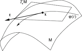
Given a point $x$ in the manifold M, and a (tangent) vector $\bf t$ in $T_x$, consider a curve that passes through $x$ in the direction of $\bf t$ described by the parameter $t$:

$x (t)$ so that $x(0) = x$, and $\frac{d x}{dt}\vert_{t=0} = {\bf t}$

With this parametrization of the curve, we can define the covariant derivate of another vector $T$ (the name $T$ is forshadowing!) as simply the rate of change of the vector along this parametrized curve $T(x(t))$:

\[\nabla_{\bf t} T = \frac{d T (x(t))}{dt}\vert_{t=0}\]

This intuition works pretty well for vector fields, so I cound end this post here like everyone else does… But that is so cheating! The hardest part, how the covariant derivative is defined for more general objects than vectors, is still unexplained! And my goal is always to uncover these hidden secrets. So let’s buckle up.

Going deeper (or step 1 on how to lose readers)

Turns out that vectors are very intuitive because they are based on visual cues that can be observed in our drawings of Euclidean geometry… Higher dimensional manifolds don’t have any of those things, so we started to invent generalizations of vectors and other geometric properties which we called Tensors (and you can learn more about them in my previous post).

Vectors correspond to what is called as 0-1 tensors, because you can write a tensor/vector as a sum over the basis of the tangent plane at the point $T_x$:

\[T = \sum\limits_{i=1}^nT_i {\bf e_i} = T_i {\bf e_i} \text{ (using Einstein sumation convention)}\]

Where the $\bf e_i$ are basis vectors of the vector space $T_x$. Therefore the parametric definition of the covariant derivative looks like:

\[\nabla_{\bf t} T = \frac{d T (x(t))}{dt} = \frac{d}{dt}(T_i {\bf e_i}) = \frac{d T_i(x(t))}{dt} {\bf e_i} + T_i \frac{d {\bf e_i}(x(t))}{dt}\] \[= \frac{\partial T_i}{\partial x^\mu}\frac{d x^\mu}{d t} {\bf e_i} + T_i \frac{d {\bf e_i}}{d x^\gamma} \frac{d x^\gamma}{d t}\]

Where we first notice that $\frac{\partial T_i}{\partial x^\mu}$ is well defined as it is just the derivative of the scalar function $T_i$ along the curve component $x^\mu$ of the curve $x(t)$.

Then we notice on the second term of the sum, that $\frac{d{\bf e_i}}{d x^\gamma}$ is a vector as well (the variation of $e_i$ along the curved trajectory), so it can be written as a sum of the basis vectors $\bf e_i$

\[\frac{d{\bf e_i}}{d x^\gamma} = \sum\limits_{j}\Gamma^j_{i\gamma} {\bf e_j}\]

where we are calling the coefficients of this sum as $\Gamma^j_{i\gamma}$, sometimes referred to as the Christoffel symbols. This is just a name for some constants, don’t freak out (not yet).

Ok so, if we put some things together, for example noticing that $\frac{d x^\mu}{d t} = t^\mu$, exchanging the indices $i$ and $j$ on the second term, and renaming the $\gamma$ and $\mu$ indices as well, we get that

\[\label{eq:cov_der_scalar} \nabla_{\bf t} T = T_{i,\mu} t^\mu {\bf e_i} + T_i \Gamma^j_{i\gamma} t^\gamma {\bf e_j} = T_{i,\mu} t^\mu {\bf e_i} + T_j \Gamma^i_{j\gamma} t^\gamma {\bf e_i} = (T_{i,\gamma} + T_j \Gamma^i_{j\gamma})t^\gamma{\bf e_i}\]

So that in terms of components, some people chose to write the covariant derivative as

\[\label{eq:misleading} \nabla_{\gamma} T = T_{i;\gamma} = T_{i,\gamma} + \Gamma^i_{j\gamma} T_j\]

but this is of course incomplete if not a little misleading too. The cruelty of geometers… (and mathematicians in general). This is what I would call an abuse of notation. It’s only allowed if you are an expert in the field. For the rest of the mortals, please write everything out!

Second step on how to lose readers

So just from this brief and intuitive analysis based on the geometric idea, we can see that we want the Covariant derivative (as described in the misleading equation) to be at least an operator that takes tangent vectors $T$ (aka 0-1 tensors), and transforms them into a 1-1 tensor.

Note: What is a 1-1 tensor anyway? In the misleading equation above, in order to complete the actual formula without abuse of notation, or better said to complete the expression so that the outcome is a scalar, one needs to “multiply” (and add with Einstein notation) the 2 terms: $t^\gamma$ and $e_i$, like in the equation for the derivative of $T$ above.

We refer to $e_i$ as a tangent vector, because as we defined it above, it is a basis vector that lives in the tangent plane $T_x$ (at the point x). This is also a 0-1 tensor.

In contrast, we consider $t^\gamma$ to be a covariant vector, or a 1-0 tensor, because in order to get a scalar one needs to “multiply” it with a 0-1 vector (like the $e_i$ for example). One can think of covariant or 1-0 tensors as linear functions on the tangent space $T_x$, as in they act/operate on vectors, like a linear function:

\[\mathbb{L}(v) = t^\gamma v_\gamma\]

Note: Why is it then that this “linear functional” is also a set of numbers $t^\gamma$ that just multiply in order to act?

Well, this comes from the fact that the only linear functionals in a vector space are constants. (This is the same reason why matrices are boxes with numbers!)

But don’t worry if you don’t grasp this right away. Thinking like this takes some time. I don’t want to encourage you skip it though, cause Physicists normally would underplay the importance of understanding that fact (that 1-0 tensors or covariant vectors are linear functions over the tangent space of vectors), but later on when one tries to look at harder material, this gap will cost you greatly.

Going even deeper: What happens if we take the covariant derivative of a covariant vector (1-0 tensor)?

First it is important to understand what are we trying to do, or what does it mean to compute the covariant derivate of a 1-0 tensor? What are we after?

We need to concretize the problem:

Say $w^i$ is a covariant vector (aka 1-0 tensor). What does it mean to derive it covariantly?

Well, the geometric idea in my mind is that now we have a field/function that is meant to operate on tangent vectors of different points in a manifold, but it acts (as a function) differently depending in which point of the manifold you are. So the covariant derivative is trying to compute the rate of change of this linear function across the manifold in some tangent vector’s direction.

Since we want to compute a derivative of $w^i$ , we have to do this at a point of the manifold $x$, and in some direction $\bf t$ that lives in the tangent plane at x, so just like before, we consider a parametrization $x^\mu (t)$ so that $\frac{d x^\mu}{dt}\vert_{t=0} = {\bf t}$. But notice that now we want to evaluate $w$ along the curve (not just at one point $x$)! The point $x$ is somewhat changing, and therefore so is the tangent plane $T_x$. This means that we actually need to choose a sequence of vectors $v(x)\in T_x$ for $x$ along the curve. Then, as we apply $w(x)$ onto $v(x)$, we get a scalar that changes along the curve, and we can take the derivative of this scalar.

With all of that context in the background, we can proceed to do the typical calculation that will give us the covariant derivative of a 1-0 tensor as it is presented everywhere.

We will choose a particularly “easy” sequence of vectors $v(x)$ though: The basis element $e_j$. This is a cool trick because their mutual application is straightforward by definition of the base elements $w^k$ of $V_x^\ast$:

\[e_j(w^k) = \delta^k_j\]

Therefore,

\[\nabla_t (e_j (w^k)) = 0\]

Remember that this is a scalar over the manifold, so we should be able to take its covariant derivative as the normal derivative along a curve that passes through the point x in the direction of $\bf t$. In a way there is a hidden dependance on the point $x$ that made explicit looks like $e_j(x(t), w^k)$. Therefore, if we apply the chain rule to the components of $x$ and then to $w$,

\[\frac{d}{dt} (e_j(x(t), w^k)) = \frac{\partial e_j}{\partial e_i} \frac{d x_i(t)}{dt} (w^k) + \frac{d e_j}{d w} (w^k) \frac{d w^k(x(t))}{dt}\]

where the term $\frac{\partial e_j}{\partial e_i}$ is an awkward way of representing the derivative of the components $e_j$ along the curve $x(t)$ (sorry, I didn’t want to use other symbols to not skip steps), but THAT IS EXACTLY THE DEFINITION OF THE COVARIANT DERIVATIVE!

The same is actually happening in the second term, where the derivative $\frac{d w^k(x(t))}{dt}$ is also the covariant derivative, now of $w$.

So we actually have:

\[= (\nabla_{e_i}e_j) (w^k) t_i + \frac{d e_j}{d w} (w^k) (\nabla_{e_i} w^k) t_i\]

where we noticed again that $\frac{d x_i(t)}{dt} = t_i$.

We can recognize a term here $(\nabla_{e_i}e_j) (w^k) = \Gamma_{ij}^l e_l (w^k) t_i$, from the definition of the Christoffel symbols, so that term is pretty solid.

Now what about the weirdo

\[\frac{d e_j}{d w} (w^k)\]

Well, this awkward symbol is representing the derivative of $e_j$ as a linear operator acting on the $w$’s, basically $e_j: V_x^\ast \rightarrow \mathbb{R}$, and this is the derivative of that operator…

But what is the derivative of a linear operator? I’ll gove you a hint, what is the derivative of $f(x) = ax$? What is the derivative of $f({\bf x}) = A{\bf x}$? That’s right! it’s the operator constant itself!! $f’ = a$ or $f’ = A$, so we can conclude that

\[\frac{d e_j}{d w} (w^k) = e_j\]

So putting this together we get

\[0 = \Gamma_{ij}^l e_l (w^k) t_i + e_j (\nabla_{e_i}w^k t_i)\]

where the second term means in words “$e_j$ applied to $\nabla_{e_i} w^k t_i$”.

Remember that we are doing this calculation because we are after the term $\nabla_{e_i} w^k$. Since this is the goal, putting a name to it can help us figure it out. Say we name it,

\[\nabla_{e_i} w^k = C_{il}^k w^l\]

since it’s a 1-0 tensor (that depends on the indices i, k), so we can write it on the basis ${w^l}$.

So finally we have

\[0 = \Gamma_{ij}^l e_l(w^k) t_i + e_j(C_{il}^k w^l t_i)\] \[0 = \Gamma_{ij}^l \delta_l^k t_i + e_j(w^l) C_{il}^k t_i\] \[-\Gamma_{ij}^k t_i = C_{ij}^k t_i\]

And since this should be true for all tangent vectors $t$, then we conclude that the coefficients $C_{ij}^k = - \Gamma_{ij}^k$, which means that the covariant derivative of a 0-1 tensor $w$ in the direction of a basis vector $e_i$ is a 1-0 tensor that looks like,

\[\nabla_{e_i} w^k = -\Gamma_{il}^k w^l\]

(remember these objects have to be evaluated on tangent vectors).

The final countdown

Now we finally made it to the final and easiest part, putting everything together.

Note: This final derivation is typically the only thing included in other reasorces and even books sometime. *Shakes fist in anger!

Anyways, lets consider a 1-1 tensor $T$, that can be described in its basis of “simple” 1-1 tensors

\[T = \sum_{i,j} T^i_j\ e_i\otimes w^j = T^i_j\ e_i\otimes w^j\]

where we are using Einstein sum notation in the last bit of the right.

So lets break it down before we try to compute the covatiant derivative of this whole thing:

\[T = \underbrace{T^i_j}_{\text{scalar}} \ \ \underbrace{\bf e_i}_{\text{covariant vector}} \otimes \ \ \ \underbrace{w^j}_{\text{tangent vector}}\]

We know how to calculate the derivative of all these things!

Let’s go:

\[\nabla_t T = \nabla_t (T^i_j e_i\otimes w^j)\\ = (\nabla_t T^i_j) e_i\otimes w^j + T^i_j (\nabla_t e_i) \otimes w^j + T^i_j e_i\otimes (\nabla_t w^j)\]

Firs term is the covariant derivative of a scalar, so it’s just a directional derivative:

\[\nabla_t T^i_j = \frac{\partial T^i_j}{\partial x^k} t_k = T^i_{j, k} \ t_k\]

The second term is the covariant derivative of a basis tangent vector, which we calculated in the second part of this article:

\[\nabla_t e_i = \nabla_{e_k} e_i\ t_k = \Gamma^l_{ik} e_l\ t_k\]

And the third term has the covariant derivative of a covariant vector (or 0-1 tensor), and it was calculated in the fourth section:

\[\nabla_t w^j = \nabla_{e_l} w^k\ t_l = -\Gamma_{lk}^j\ w^l\ t_k\]

Then putting it all together:

\[\nabla_t T = T^i_{j, k} \ t_k\ (e_i\otimes w^j) + T^i_j\ \Gamma^l_{ik}\ (e_l\ \otimes w^j)\ t_k - T^i_j\ \Gamma_{lk}^j\ (e_i\otimes \ w^l)\ t_k\\ = t_k [T^i_{j,k} + T^l_j \Gamma^i_{kl} - T^i_l \Gamma^l_{kj}] (e_i\otimes w^j)\]

People would then write this omitting all the complexity like this:

\[\nabla_t T = T^i_{j,k} + T^l_j \Gamma^i_{kl} - T^i_l \Gamma^l_{kj}\]

but this is hopefully now an obvious omission of context and clear abuse of notation (which will keep us enraged until we dominate this material a little more.. perhaps…)

Conclusion

Now that we know how to compute the covariant derivatives of all basis elements of both $V_x$ and $V_x^\ast$, we saw above that we have the power to compute it for 1-1 tensors using that magical basis ${e_i\otimes w^j}$

But we are actually capable of extending this result for any tensor rank possible… we just need to write this tensor in that magical basis, and apply the product rule over and over and over, until all the factors of the basis $e_1\otimes\dots\otimes e_n \otimes w^1 \otimes \dots \otimes w^n$ are taken care of.

I’m not going to write it here but you get the idea.

Calculating these beasts seams almost attainable now… perhaps one might even venture that it is “mechanic”… But the secret is that understanding of the layers hiding behind the process is trickier than advertised, so I hope this article helps demystify what is going on a little bit.

Maybe next time we could review some calculations of real tensors (like the metric tensor, or the Energy-Momentum tensor from Electromagnetics) to concretize what we have covered today! Let me know in the comments what you think.

Happy covariant-derivating!

---

Comments

Join the discussion for this article by clicking Here. Comments appear on this page instantly.

No comments found for this article.